What is "2-point" KestrelCalTM calibration?

The "2-point" calibration method was developed exclusively by Catalina Scientific for use with the SE 200 echelle-type spectrograph built by Optomechanics Research.

To calibrate an SE 200, an Hg image is first acquired and any two prominent Hg peaks are selected for the 2-point calibration. KestrelSpec has a Peak Finder tool for images to aid in determining the location of prominent peaks. Below is an example of an Hg echelle image with the prominent peaks labeled:

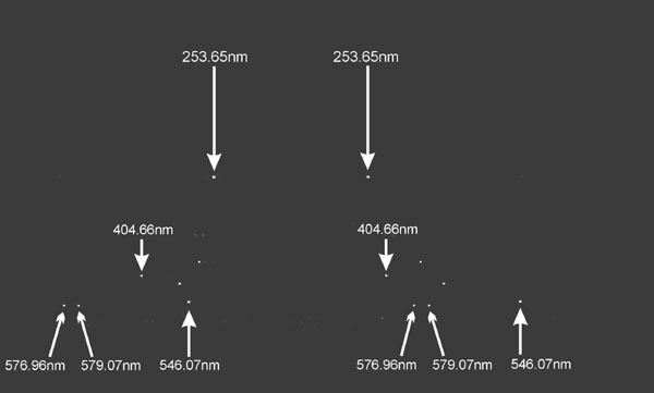
The X and Y coordinates of two prominent Hg peaks are entered in the calibration dialog box, which in this example are 546.074nm and 579.066nm for an SE 200 spectrograph:

The user then clicks on the Calibrate X Axis button and KestrelSpec calculates the calibration parameters that will be used in the creation of spectral curves from acquired images. Once the "2-point" procedure is successful, each acquired spectral curve will be accurately calibrated in either nm or Raman cm-1 units.

What is "3-point" KestrelCalTM calibration?

The "3-point" calibration method was developed exclusively by Catalina Scientific for use with the EMU-120/65 echelle spectrograph that we design and build.

To calibrate the EMU-120/65 spectrograph, an Hg/Ar image is first acquired and three prominent Hg and Ar peaks are selected for the 3-point calibration. KestrelSpec has a Peak Finder tool for images to aid in determining the location of prominent peaks. Below is an example of an Hg/Ar echelle image acquired with the EMU-120/65 with the prominent peaks labeled:

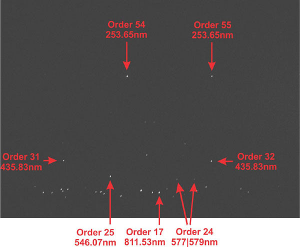
The X and Y coordinates of three prominent Hg and Ar peaks are entered in the calibration dialog box, which in this example are two Hg peaks at 253.652nm and an Ar peak at 811.531nm:

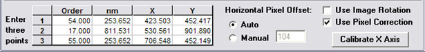
The user then clicks on the Calibrate X Axis button and KestrelSpec calculates the calibration parameters that will be used in the creation of spectral curves from acquired images. Once the "3-point" procedure is successful, each acquired spectral curve will be accurately calibrated in either nm or Raman cm-1 units.

What is KestrelTempTM temperature calibration?

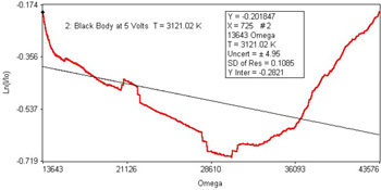
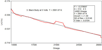
In the current version of the KestrelSpec software, there is an option to acquire and display spectral curves in Temperature Mode. KestrelTempTM is a method of calculating the unknown temperature of spectral data once a temperature reference curve, with a known temperature, has been defined. This known temperature reference curve and any unknown sample curve are then transformed by a proprietary algorithm to produce a linear function of relative intensity versus frequency (Omega). The temperature of the unknown source can then be calculated from the slope of this relationship between relative intensity and frequency. The software calculates a least squares fit to the function and determines the temperature of the unknown source including a 1 sigma error coefficient. The accuracy of the temperature calculation can be optimized by adjusting the spectral range over which the least squares fit is operating. The better the fit, the smaller the temperature error estimate.

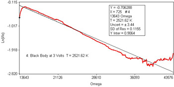
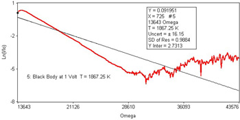
In the sample temperature spectra below, a reference spectrum was acquired from 330nm to 1050nm using a black body source at 6 volts with a known temperature of 3200K. Three subsequent spectra of unknown temperature were then acquired covering the same 330nm to 1050nm range using the black body source at 5, 3 and 1 volts. The curves below show the relative intensity versus frequency and the calculated temperature and error estimate for each of the unknown samples:

The user can toggle back and forth between standard spectral mode with wavelength or Raman units along the X axis, and temperature mode with Omega units along the X axis.

	The black body at 5 volts has a temperature of 3121.02 K with an error estimate of +/- 4.95 for the full 330nm to 1050nm range. The wavelength range corresponds to an Omega range from approximately 13643 to 43576. The fit can be greatly improved by limiting the Omega range.
	This example shows how the black body at 5 volts has a temperature of 2991.67 K with an error estimate of +/- 1.49 by limiting the frequency range of the fit. The Omega range in the above example has been reduced to go between 14000 to 28000, which corresponds to a wavelength range of about 340nm to 680nm.
	The black body at 3 volts has a temperature of 2521.62 K and an error estimate of +/- 3.44 for the full 330nm to 1050nm range. A better fit, and a lower error estimate, can be achieved by limiting the Omega frequency range from 13643 to about 36100.
	The black body at 1 volt has a temperature of 1867.25 K for the full 330nm to 1050nm range with an error estimate of +/- 16.15, which is the highest of the three samples at 5, 3 and 1 volts. By decreasing the Omega range to include only the linear portion of this 1 volt curve, the fit can be improved.
What is the Element Identification process? In the current version of the KestrelSpec software, there is an option to identify common elements in spectral curves, which is ideal for LIBS (laser-induced breakdown spectroscopy). There is an Element Identification option on the main Process menu that allows the user to search for elements in any spectral curve that is calibrated in nm units. Here is an example of element identification:
	In this example, the KestrelSpec software searched the spectral data of a penny coin for all the elements in the periodic table. Elements are identified according to the number and intensity of known peaks in each element. The built-in Peak Finder looks for peaks in the spectral data according to user-adjustable parameters like the threshold of peak intensity, its wavelength tolerance, and the minimum number of peaks to find for each identified element. The user can also adjust the wavelength range for the element search, which in this sample for the penny coin was 200nm through 520nm. The search in the given wavelength range with the user-entered thresholds and tolerances for the peak finder found two prominent elements in the penny coin: Cu with 10 peaks Zn with 6 peaks These peak results are just a summary. More details can be viewed and saved to a file, as shown below.
	The 10 peaks of Cu and the 6 peaks of Zn found in the sample curve named Penny are displayed sorted by Sample Intensity, which is the last column labeled Samp Intens. All of these peaks are within the user-entered wavelength range of 200nm through 520nm. The identified sample peaks in each element can be sorted either by the Reference Wavelength (nm) or by the Sample Intensity. Both the wavelength and the intensity of each Reference and Sample peak are displayed. By default, the NIST reference tables are used for identification, but KestrelSpec is flexible and allows reference tables to be user-defined.
	By clicking on the Sort by Reference (nm) button, the identified peaks of Cu and Zn are displayed sorted by reference wavelength, which is the column labeled Ref (nm). The detailed results for the peaks found in the identified elements can be scrolled in the display window. These results can also be saved to a file that can then be imported into a spreadsheet or a data analysis program.